
Chapter 8: ML Perceptrons
ML Perceptrons (or just Perceptron in Machine Learning). This is one of the most important topics because it’s the building block of every modern neural network — from simple classifiers to today’s massive deep learning models like the ones powering me (Grok)!
I’ll explain it step-by-step like a patient teacher: no rush, lots of intuition, real examples (including the famous logical gates), diagrams via pictures, and why it’s still taught even in 2026.
Step 1: What Exactly is a Perceptron?
A Perceptron is the simplest artificial neuron — the most basic unit in a neural network.
- Invented by Frank Rosenblatt in 1957–1958 (inspired by how real brain neurons work).
- It’s a binary classifier: It decides “yes” (1) or “no” (0) — like “Is this email spam?” or “Is this tumor malignant?”
- It’s supervised learning — we give it examples with correct answers, and it learns by adjusting itself.
Think of it as a tiny decision-maker inside your brain: it gets signals (inputs), weighs how important each signal is, adds them up, and if the total is strong enough → it “fires” (says 1), else stays quiet (says 0).

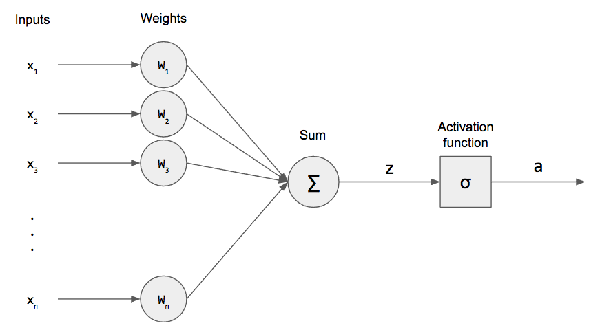
Look at these diagrams — this is the classic single perceptron:
- Left side: Inputs (x₁, x₂, x₃, …) come in
- Each has a weight (w₁, w₂, …) — like importance score
- Weights multiply inputs → sum them up (weighted sum) + a bias (b) to shift the decision
- Then pass through a step function (activation) → output 0 or 1
Math (simple version):
z = (w₁ × x₁) + (w₂ × x₂) + … + b Output ŷ = 1 if z ≥ 0, else 0
(Modern versions sometimes use sign function or sigmoid, but classic perceptron uses hard step.)
Step 2: Famous Real Example – Learning Logical Gates (AND Gate)
The perceptron shines when learning simple rules like logic gates — because gates are binary decisions.
Let’s take the AND gate (only outputs 1 if BOTH inputs are 1):
Truth table:
| Input A (x₁) | Input B (x₂) | Output (y) |
|---|---|---|
| 0 | 0 | 0 |
| 0 | 1 | 0 |
| 1 | 0 | 0 |
| 1 | 1 | 1 |
We want perceptron to learn: “Fire (1) only if both A and B are 1”.
We can do this with:
- Weights: w₁ = 0.7, w₂ = 0.7
- Bias: b = -1.0 (or threshold around 1)
Let’s calculate for each case:
- x₁=0, x₂=0 → z = 0.70 + 0.70 -1 = -1 < 0 → output 0 ✓
- x₁=0, x₂=1 → z = 0.70 + 0.71 -1 = -0.3 < 0 → output 0 ✓
- x₁=1, x₂=0 → z = 0.71 + 0.70 -1 = -0.3 < 0 → output 0 ✓
- x₁=1, x₂=1 → z = 0.71 + 0.71 -1 = 0.4 ≥ 0 → output 1 ✓
Perfect! It learned the AND rule.

See? The weighted sum + bias creates a decision boundary — a straight line in 2D that separates the points where output=1 from output=0.
Step 3: How Does the Perceptron Actually Learn? (The Magic Part)
It starts with random weights (say all 0).
Then it follows the Perceptron Learning Rule (very simple update):
For each training example (x, true y):
- Make prediction ŷ
- If correct → do nothing
- If wrong → adjust weights!
Update rule:
- If predicted 0 but should be 1 → increase weights toward this example: w_new = w_old + learning_rate × x
- If predicted 1 but should be 0 → decrease weights: w_new = w_old – learning_rate × x
- Bias updates similarly.
Repeat over all examples many times (epochs) → weights slowly move until all points are correctly classified (if possible).
Key guarantee (Perceptron Convergence Theorem): If data is linearly separable (can be split by a straight line/plane), the algorithm will find perfect weights in finite steps!
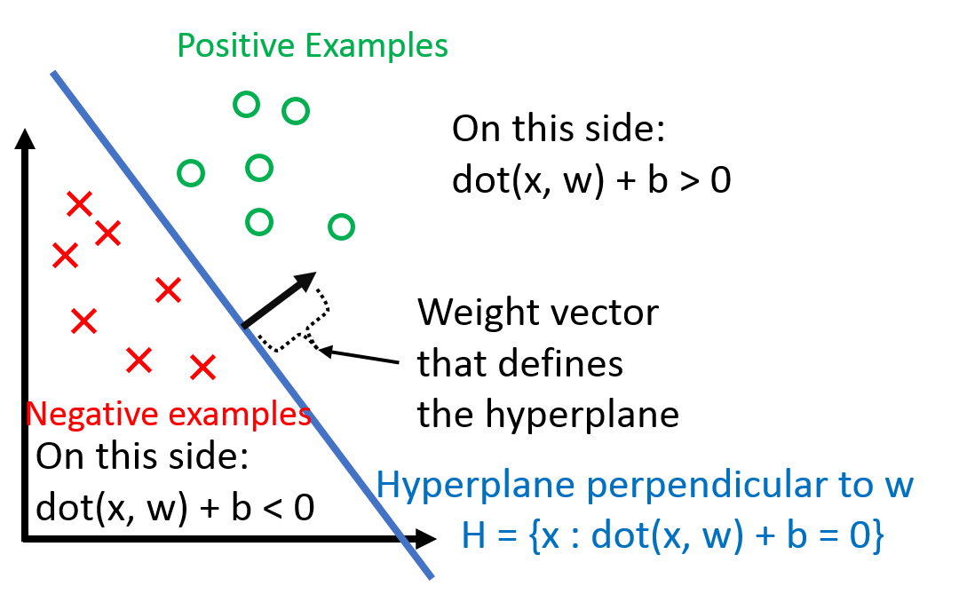
This picture shows how the boundary (hyperplane) moves during updates until it separates green (+) and red (-) points perfectly.
Step 4: Limitations – Why We Needed More (Multilayer Perceptrons)
Perceptron can only learn linearly separable problems.
It cannot learn XOR gate:
| A | B | XOR |
|---|---|---|
| 0 | 0 | 0 |
| 0 | 1 | 1 |
| 1 | 0 | 1 |
| 1 | 1 | 0 |
No straight line can separate the 1’s from 0’s — they form a diagonal pattern.
This limitation (shown by Minsky & Papert in 1969) killed single-layer perceptron hype for years… until people added hidden layers → Multilayer Perceptron (MLP) → deep neural networks!
Quick Summary Table (Copy This!)
| Part of Perceptron | What it Does | Example in AND Gate |
|---|---|---|
| Inputs (x₁, x₂, …) | Features/data points | A and B (0 or 1) |
| Weights (w) | Importance of each input | 0.7 for both |
| Bias (b) | Shifts the decision threshold | -1.0 (needs strong signal to fire) |
| Weighted Sum (z) | Total evidence | w₁x₁ + w₂x₂ + b |
| Activation (Step) | Final decision (0 or 1) | 1 only if z ≥ 0 |
| Learning Rule | Adjusts weights on mistakes | +x if under-predict, -x if over |
| Limitation | Only linear boundaries | Can’t do XOR |
Final Teacher Words (2026 Perspective)
The perceptron is like the “wheel” of ML — simple, but everything complex (ChatGPT, image generators, self-driving) is built by stacking millions of them with better activations (ReLU, sigmoid), layers, and training tricks (backpropagation, Adam).
In 2026, we rarely use single perceptrons alone — but understanding it deeply helps you debug why a big model fails, or why a problem needs non-linearity.
Got it? 🌟
Questions?
- Want Python code to build AND/OR/XOR perceptrons yourself?
- How multilayer perceptrons fix XOR?
- Difference between perceptron vs modern neuron (sigmoid vs step)?
Just say — next class is ready! 🚀


